Lab 10

Blogsheet week 10

In this week’s lab, you will collect more data on low pass and high pass filters and “process” them using MATLAB.

PART A: MATLAB practice.
Open MATLAB. Open the editor and copy paste the following code. Name your code as FirstCode.m

Save the resulting plot as a JPEG image and put it here.

clear all;

close all;

x = [1 2 3 4 5];

y = 2.^x;

plot(x, y, 'LineWidth', 6)

xlabel('Numbers', 'FontSize', 12)

ylabel('Results', 'FontSize', 12)

This is an image of the plot we got with the above MATLAB code

       What does clear all do?

          Clear all clears all data and objects from the work space and closes the MuPAD engine which resets all of the programs assumptions.

       What does close all do?

          The close all function deletes all figured whose handles are not hidden.

       In the command line, type x and press enter. This is a matrix. How many rows and columns are there in the matrix?

          1 row 5 columns.

       Why is there a semicolon at the end of the line of x and y?

          When you are defining component equations you have to end the functions with a semicolon otherwise it will result in an error.  MATLAB needs the semicolon so it knows that is a function or definition, if you do not do this it results in an error message displaying an "unexpected MATLAB expression".

       Remove the dot on the y = 2.^x; line and execute the code again. What does the error message mean?

          The error message means that we are giving x values in vector quantities and our y is trying to display scalar quantities so if we put the dot before the exponent it will result in a vector output.

       How does the LineWidth affect the plot? Explain.

          The LineWidth 1 is equal to having a simple plot of x and y.  If you keep increasing the line width it increases the thickness of the line, possibly to make it easier to differentiate from others in the same plot.

       Type help plot on the command line and study the options for plot command. Provide how you would change the line for plot command to obtain the following figure (Hint: Like ‘LineWidth’, there is another property called ‘MarkerSize’)

Fig. 1

             You would alter the line for the plot to "plot(x, y, '-ro', 'LineWidth', 4, 'MarkerSize', 16)"

       What happens if you change the line for x to x = [1; 2; 3; 4; 5]; ? Explain.

       From what we can tell nothing changes in the plot that the code executes.  Basically the semi-colon defines all the numbers in the brackets to x.  When you add a semi-colon behind each number it is doing the same thing, but in a different way.

       Degree vs. radian in MATLAB:

a.       Calculate sinus of 30 degrees using a calculator or internet.
       sin(30) = .5

b.      Type sin(30) in the command line of the MATLAB. Why is this number different? (Hint: MATLAB treats angles as radians).

      This number is different because when you use a calculator or the internet it generally calculates sin as a degree, while MATLAB gives answers as rads.

c.       How can you modify sin(30) so we get the correct number?

       sin(30*2*pi/360)

2      Plot y = 10 sin (100 t) using Matlab with two different resolutions on the same plot: 10 points per period and 1000 points per period. The plot needs to show only two periods. Commands you might need to use are linspace, plot, hold on, legend, xlabel, and ylabel. Provide your code and resulting figure. The output figure should look like the following:

Fig 2.

Code:

clear all;

close all;

t1 = linspace(0, (4*pi)/100, 10);

t2 = linspace(0, (4*pi)/100, 1000);

y1 = 10*sin(100*t1);

y2 = 10*sin(100*t2);

plot(t1, y1, '-ro', t2, y2)

xlabel('Time (s)')

ylabel('y function')

legend('course', 'fine')

Our graph generated by the code above

       Explain what is changed in the following plot comparing to the previous one.

Fig. 3

         In the graph in figure 3, the coarse line remains the same as in fig. 2 and the fine line differs from fig.2 because it is clipping the top of the sinusoidal line.

        The command find was used to create this code. Study the use of find (help find) and try to replicate the plot above. Provide your code.

PART B: Filters and MATLAB

       Build a low pass filter using a resistor and capacitor in which the cut off frequency is 1 kHz. Observe the output signal using the oscilloscope. Collect several data points particularly around the cut off frequency. Provide your data in a table.

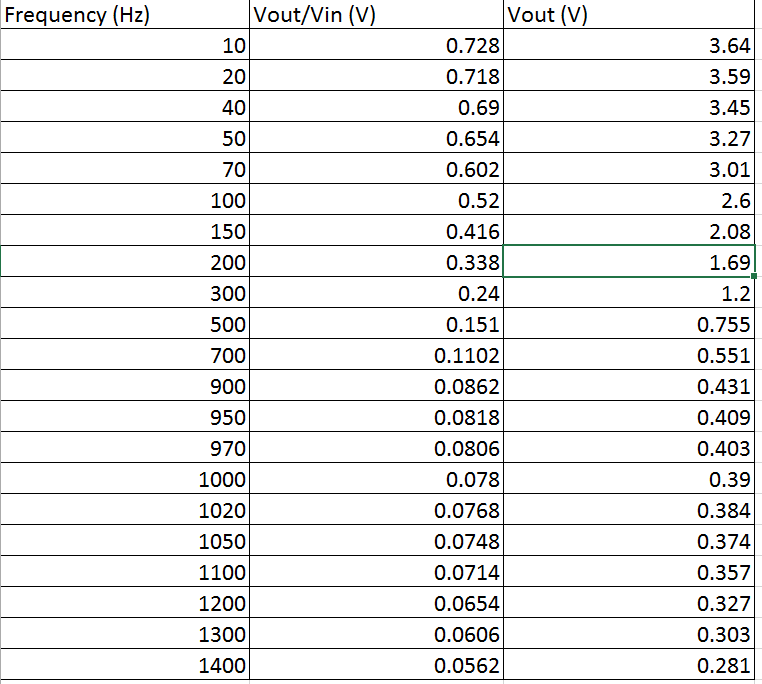Our values for the low pass filter

       Plot your data using MATLAB. Make sure to use proper labels for the plot and make your plot line and fonts readable. Provide your code and the plot.

clear all;

close all;

Frequency = [10 20 40 50 70 100 150 200 300 500 700 900 950 970 1000 1020 1050 1100 1200 1300 1400];

LPvoltage = [3.64 3.59 3.45 3.27 3.01 2.6 2.08 1.69 1.2 0.755 0.551 0.431 0.409 0.403 0.39 0.384 0.374 0.357 0.327 0.303 0.281]

HPvoltage = [0.356 0.692 0.885 1.57 2.01 2.49 2.94 3.17 3.38 3.5 3.57 3.58 3.64 3.63 3.58 3.55 3.53 3.58 3.58 3.58 3.58]

plot (Frequency, LPvoltage, 'o-r')

hold on;

plot (Frequency, HPvoltage, 'o-b')

hold on;

xlabel('Frequency (Hz)')

ylabel('Vout (V)')

legend('Low Pass', 'High Pass')

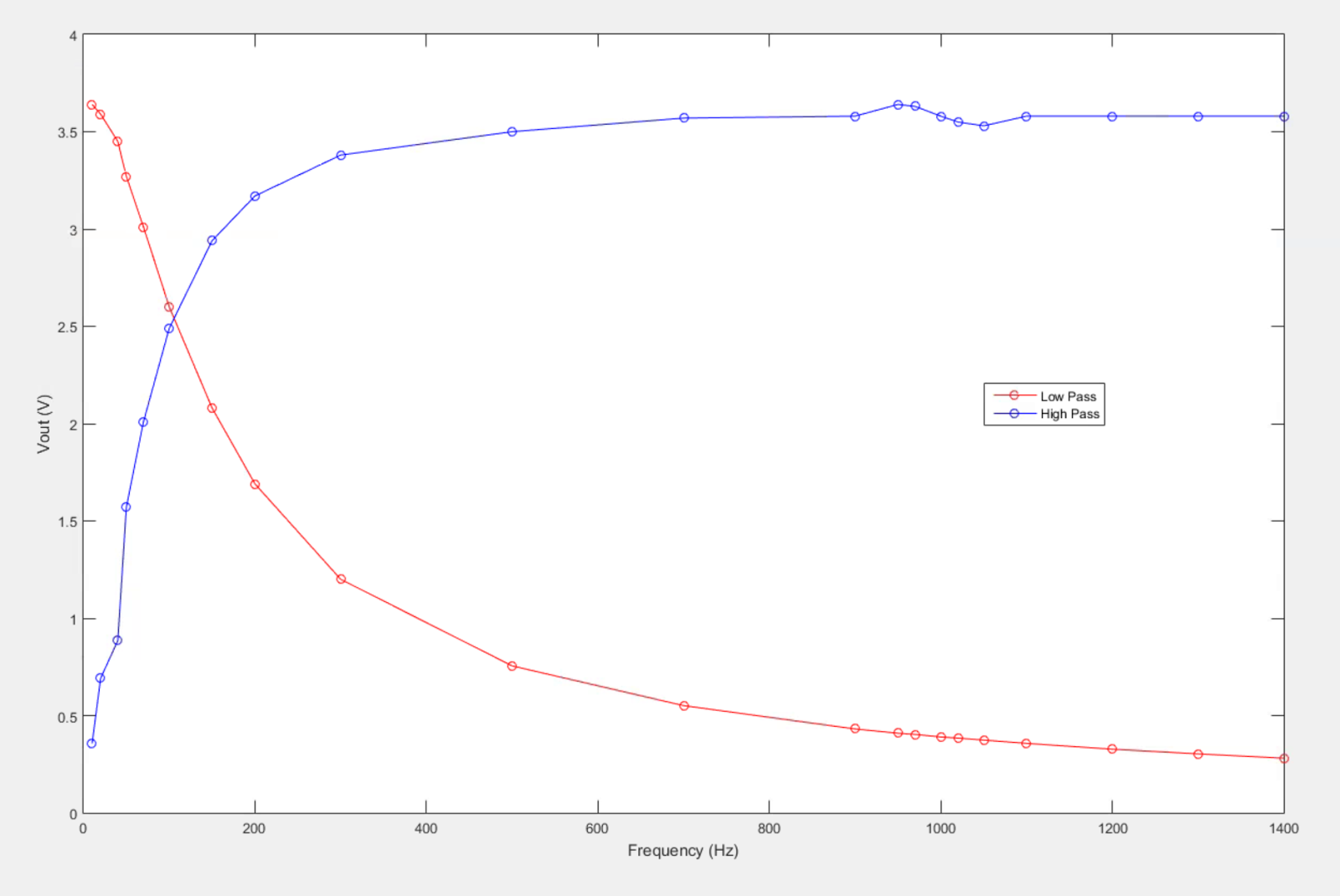The plot of both our High Pass and Low Pass filters

       Calculate the cut off frequency using MATLAB. find command will be used. Provide your code.

clear all;

close all;

Frequency = [10 20 40 50 70 100 150 200 300 500 700 900 950 970 1000 1020 1050 1100 1200 1300 1400];

LPvoltage = [3.64 3.59 3.45 3.27 3.01 2.6 2.08 1.69 1.2 0.755 0.551 0.431 0.409 0.403 0.39 0.384 0.374 0.357 0.327 0.303 0.281]

plot (Frequency, LPvoltage, 'o-r')

hold on;

xlabel('Frequency (Hz)')

ylabel('Vout (V)')

legend('Low Pass')

y = find(LPvoltage<(.707*5));
for n=1: length(y)
    m(n)= y(n)
    a(n)= Frequency(m(n))
end
fcLP = max(a(n))
plot([fcLP,fcLP], [0,4], '--r');

       Repeat 1-3 by modifying the circuit to a high pass filter.

Our values for the high pass filter

clear all;
close all;
Frequency = [10 20 40 50 70 100 150 200 300 500 700 900 950 970 1000 1020 1050 1100 1200 1300 1400];
HPvoltage = [0.356 0.692 0.885 1.57 2.01 2.49 2.94 3.17 3.38 3.5 3.57 3.58 3.64 3.63 3.58 3.55 3.53 3.58 3.58 3.58 3.58]
plot (Frequency, HPvoltage, 'o-b')
hold on;
xlabel('Frequency (Hz)')
ylabel('Vout (V)')
legend('High Pass')
x = find(HPvoltage<(.707*5));
for n=1: length(x)
    m(n)= x(n)
    z(n)= Frequency(m(n))
end
fcHP = max(z(n))
plot([fcHP,fcHP], [0,4], '--b');

Lab 9

Blogsheet week 9

1.  Measure the resistance of the speaker. 

       It keeps fluctuating between 7.9 and 8.2.

2. Build the following circuit using a function generator setting the amplitude to 5V (0V offset). What happens when you change the frequency? (video)

Fig 1. Test setup for the speaker.

Fill out the following table.

Frequency (kHz)	Observation
1	Steady squeal
2	Lower pitched tone
3	Higher pitched whine
4	Even more annoying
5	Most annoying

3.  Add one resistor to the circuit in series with the speaker (first 47 Ω, then 820 Ω). Measure the voltage across the speaker. Briefly explain your observations.

Voltage with the 47 Ohm resistor:  375 mV(rms) (1 kHz)

Voltage with the 820 Ohm resistor:  54 mV(rms) (1 kHz)

We noticed immediately that the pitch of the tone is lower as we make the resistor bigger.  The volume also decreases the higher the resistance.

Fill the following table.

Resistor Value (Ω)	Oscilliscope Output (Vrms)	Observation
47	0.396	Low pitched hum
820	0.054	A quiet low pitched hum

4.     Build the following circuit. Add a resistor in series to the speaker to have an equivalent resistance of 100 Ω. Note that this circuit is a high pass filter. Set the amplitude of the input signal to 8 V. Change the frequency from low to high to observe the speaker sound. You should not hear anything at the beginning and start hearing the sound after a certain frequency. Use 22 nF for the capacitor.

Fig. 2 Test setup for high pass filter

a.       Explain the operation.  (video)

b.      Fill out the following table by adding enough (10-15 data points) frequency measurements. Vout is measured with the DMM, thus it will be rms value.

Frequency (Hz)	Vout (Vrms)	Vout(rms) / Vin(rms)
1000	0.0854	0.0106
42000	2.64	0.33
56000	3.04	0.38
83000	3.46	0.433
100000	3.58	0.448
160000	3.87	0.484
233000	4.05	0.506
308000	4.13	0.516
377000	4.22	0.528
410000	4.27	0.534
500000	4.46	0.558
801000	5.77	0.721
901000	6.6	0.825

c.       Draw Vout/Vin with respect to frequency using Excel.

Vout/Vin with frequency as the x-axis and the vout/vin as the y-axis

d.      What is the cut off frequency by looking at the plot in b?
          901 kHz

5.     Design the circuit in 4 to act as a low pass filter and show its operation. Where would you put the speaker? Repeat 4a-g using the new designed circuit (e, f, and g are for blogI).

        For the low pass filter you would connect the speaker across the capacitor much like you connect the oscilloscope. 

a.  Explain the operation (video)

b.  Fill out the following table by adding enough (10-15 data points) frequency measurements.  Vout is measured with the DMM, thus it will be the rms value.

Frequency (Hz)	Vout (rms)	Vout (rms) / Vin (rms)
679	5.9	0.738
1000	5.99	0.749
6000	5.8	0.725
15000	5.6	0.7
23000	5.3	0.663
46000	4.3	0.538
52000	4.09	0.511
57000	3.89	0.486
66000	3.57	0.446
77000	3.22	0.403
85000	2.98	0.373
92000	2.8	0.35
121000	2.26	0.283
151000	1.86	0.233

c.  Draw Vout/Vin with respect to frequency using excel.

Vout/Vin charted with frequency as the x axis and vout/vin as the y axis

d.  What is the cut off frequency by looking at the plot in b?

5.6 kHz

6.       Construct the following circuit and test the speaker with headsets. Connect the amplifier output directly to the headphone jack (without the potentiometer). Load is the headphone jack in the schematic. “Speculate” the operation of the circuit with a video.

Lab 8

Blogsheet week 8

Rube Goldberg Take 2

Draw and explain a Rube Goldberg design that will include the following components:

·       Digital

·       Motor

·       Relay

·       Opamp

·       Temperature sensor

·       LED

The setup should be considered to last 30 seconds.

Make sure to include enough photos, videos, and explanations for each “transition” or step. Explain your circuits. Put at least 2 issues/problems/struggles you faced during the project.

          For our Rube Goldberg design we decided make a design that would pull a paper flag up a flagpole and, when the timing was right, break the circuit so the motor pulling both strings would stop.

         We kept the same design and setup for the week 7 lab which we didn't disassemble after we finished and added on an OpAmp, Temp sensor, relay, and a larger motor.  The reason we used another motor wasn't because we didn't have enough power to pull the flag or to pull the wire out of the bread board, but because it had 2 axels which could be more easily utilized to pull two things at once.

The drawing of our complete circuit, including values for resistors and voltage sources

               Once we decided what we wanted to do we pulled out our week 7 design and added the OpAmp, relay, temp sensor, transistor, and motor. 

Our set up near the beginning of the project.

         We decided that we wanted the design to be completely automatic once we had set it in motion, so we decided that we would use a domino like effect to land something on the pressure sensor to start the clock and begin the process of pulling up the flag.  Since we wanted it to be fully automatic we didn't use a heat source (though we decided we might have to if we wanted to speed it up in any way or if we needed to get more voltage to the motor) so we configured the OpAmp to produce enough voltage after the temp sensor to run the motor.  Once of our biggest struggles was figuring out which resistors to use with the OpAmp to produce the desired power and speed so we could reach the 30 second minimum. 

The next iteration of our machine before we decided on another arrangement. 

        For our XOR gate we used a constant input of 1 from the 5V source and then we used the A output from the display driver (alternating between 0 and 1 every second)  to give us the right timing.  The LED would turn on while the motor was running and would turn off when it wasn't.  This was another area where we had an issue, we found that any of the inputs (B, C, or D) from the display drivers that let the motor run for more than a second at a time was too fast for the 30 second threshold. 

        The video above shows our rearranged machine using C as the output of the display driver, it moves much too fast for the 30 second threshold so we needed to rethink the output that we were going to use. 

       Another challenge for our machine was that the motor had just enough power to turn at the speed we wanted, so any additional force on the string would cause the motor not to turn.  In the video below the motor doesn't turn, and the reason for that is that the "guide" for the string, so that it wouldn't fall off track and not wind around the motor, was catching.

      After this we changed the guides so that they wouldn't hamper the progress of the string so we could get the timing down without additional difficulties.  In the end we got it nearly to what we wanted, the video below is when we demonstrated it for the class.

A picture of our completed operation

Engineering Rules!